ResNet, ResNeXt, RegNet,… what else?

The ResNet was introduced in the paper¹ “Deep residual learning for image recognition” by Kaiming He et al. in 2015. So what is the problem that its design was trying to solve? My first thought was that it improves gradient flow and allows for easier training of much deeper models, but that’s not it. The problem with vanishing/exploding gradients was already solved with techniques like batch normalization² and smart weight³ initialization⁴.

There is however a more subtle problem with designing deeper networks. And that is: How do we know that a deeper network would fit the data better? And this is not about larger models overfitting the data and performing worse. We are talking about the accuracy of the model during training. Experiments show that performance actually starts to degrade when networks become too deep, as shown on the figure:

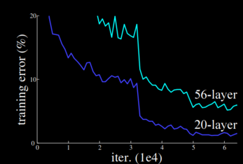
In theory, the deeper network should be able to learn the function represented by the shallower network – the last 36 layers should simply be reduced to an identity mapping. However, it turns out that, using current gradient based methods, it is not that easy to make some arbitrary part of a highly non-linear network learn to simulate the identity function. Thus, if we simply stack more layers, then we might not be able to recover solutions achievable with fewer layers. And so it might happen that deeper networks actually have higher training error.

(Note that we might simply be having issues optimizing the larger model because batch norm and weight init are not doing a good job :? But the assumption is that they are doing a good job.)

THE RESIDUAL BLOCK: EMPOWERING DEEPER NETWORKS⌗

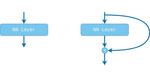
Simply stacking one more layer on top of our current model results in applying a function $F(x)=f(x)$ to the output of our model $x$. The paper proposes to change the wiring of our network by adding a shortcut connection so that $F(x)=f(x)+x$. Now if the deeper model wants to reproduce the shallower model we simply have to learn that the residual is $f(x)=0$, i.e., push the weights to 0. And the hypothesis is that learning $f(x)=0$ should be much easier than learning $f(x)=x$.

So after every conv layer we add this shortcut connection? Well, they decided to add it after every two $3 \times 3$ conv layers, following the design of the VGG block. Later experiments performed in [⁵] show that stacking two $3 \times 3$ conv layers works best.

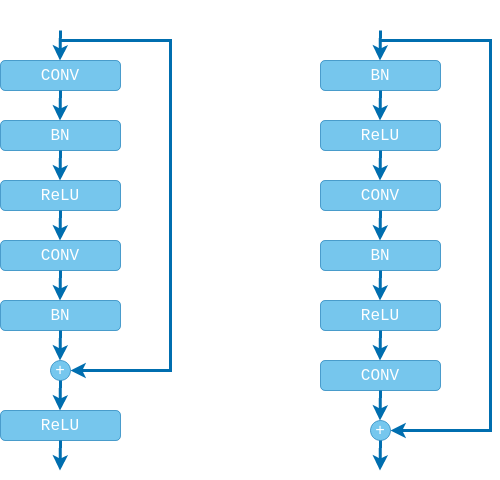
Also, don’t forget that we need to add batch normalization and non-linearity layers after every convolution. All of these layers combined, together with the shortcut connection, make the residual block (shown on the left side of the figure below). Note that the second $ReLU$ is applied after adding the shortcut connection, otherwise the residual function $f(x)$ would be strictly non-negative, while we want it to take values in $(-\infty, \infty)$. Further research however showed that this is not the optimal arrangement and for very deep networks (100+ layers) gradient flow is improved when the non-linearity is applied only to the residual branch. In their follow-up paper⁶ the authors propose a re-arrangement of the layers addressing this issue while also making the residual function $f: \mathcal{R} \rightarrow \mathcal{R}$ (shown on the right side of the figure below).

THE BOTTLENECK BLOCK: REDUCING COMPUTATIONAL OVERHEAD⌗

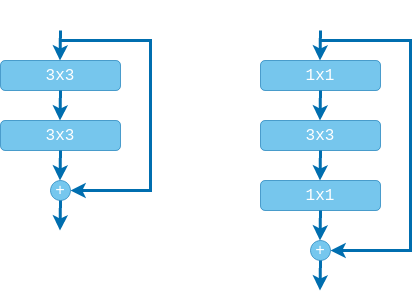
Since training deep networks could be very expensive the original paper proposes a so-called “bottleneck” block for all models deeper than 50 layers. Instead of two $3 \times 3$ layers, a stack of three layers is used: $1 \times 1$, $3 \times 3$, $1 \times 1$. The first $1 \times 1$ layer reduces the number of channels (usually in half) and the $3 \times 3$ layer is a bottleneck operating with the smaller number of input and output channels. Finally, the second $1 \times 1$ layer restores the channels back to the input size. Here, again, we have the option of arranging the batch norm and relu layers in the original arrangement or in the ‘pre-activation’ arrangement, although I think that ‘pre-activation’ is more common.

Note that the second $1 \times 1$ layer actually serves a dual purpose. In addition to up-scaling the channels it is also used to create a micro-network.

A single $3 \times 3$ conv layer is a linear filter that applies a linear transformation to the input data. In the paper⁷ “Network in network”, by Lin et al. the authors argue that it would be beneficial to replace the single conv layer with a “micro-network” structure acting on the same $3 \times 3$ patch. Now, instead of sliding a linear kernel along the image, we will be sliding the entire “micro-network”. Practically, this idea is realized by stacking $1 \times 1$ layers on top of the $3 \times 3$ layer. In our case we have one $1 \times 1$ layer resulting in a two-layer fully connected micro network.

THE RESNEXT BLOCK: GOING WIDER INSTEAD DEEPER⌗

Using the ResNet block we can create super deep models (think ~1000 layers) and now the performance of the model will not degrade. But will it improve? Well, no. Stacking more layers will improve performance up to some point and beyond that we only get diminishing returns.

Another way to improve performance is to go wider instead of deeper. What this means is, instead of stacking more layers, we increase the number of channels in each of the convolutional layers. This effectively makes our networks learn features in higher dimensional spaces. This idea is thoroughly explored in the paper⁵ “Wide residual networks” by Zagoruyko and Komodakis. A wider network having 50 layers but twice the channels in each of these layers outperforms the ResNet-152 on ImageNet.

Unfortunately, increasing the number of channels increases the computational costs quadratically (not speed! since it’s parallelizable). To fix this problem the ResNeXt block was proposed in the paper⁸ “Aggregated residual transformations for deep neural networks” by Xie et al. The idea follows the split-transform-merge strategy:

• we first split the channels $C$ of the input into $g$ independent groups;
• we then apply different convolutional transformations to each of the groups producing $g$ outputs, i.e., grouped convolution (supported by DL frameworks);
• and, finally, we aggregate the results by concatenating.

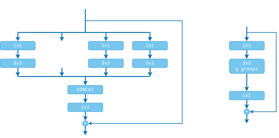
The idea of splitting the computation into several groups was inspired by the Inception network⁹. However, instead of having every branch perform a different computation (e.g. $3 \times 3$ conv, $5 \times 5$ conv, etc.), the ResNeXt block performs the same transformation in all branches. This increases modularity and reduces the number of hyper-parameters that need to be tuned. Using this approach we greatly reduce the computational costs and the number of parameters while still allowing for wider networks. Moreover, the authors report that, instead of simply creating wider networks, it is better to divide the channels into groups.

The downside is that the channels are split into independent groups and no information is exchanged between them until the final aggregation operation. For this reason we sandwich the grouped convolution between two $1 \times 1$ conv layers, making the ResNeXt block look a lot like a bottleneck block, but for entirely different reasons. In the bottleneck block the $1 \times 1$ conv layers are used for reducing and subsequently increasing the channels, thus making the $3 \times 3$ conv a bottleneck. Here, however, the $1 \times 1$ conv layers are used for intermixing the information along the channels before and after applying the grouped convolution. We don’t have to reduce the channels and have the $3 \times 3$ grouped conv behave like a bottleneck. In fact, the results of [¹⁰] show that both reducing (bottleneck) and increasing (inverted bottleneck) channels degrades the performance.

At the extreme you could use $g=C$ as proposed in [¹¹], which means having each group contain only one channel. Combining this with a $1 \times 1$ convolution afterwards leads to the famous depthwise separable convolution. This combination leads to a separation of spatial and channel mixing, where each operation either mixes information across spatial or channel dimension, but not both. This approach greatly reduces the number of parameters in the model, but may also harm accuracy.

THE ARCHITECTURE OF THE RESNET⌗

So the ResNet is constructed by stacking residual blocks one after another, but there are a few subtleties. A typical conv network is divided into stages and in each stage several residual blocks are applied, operating on fixed dimensions $C \times H \times W$ (note that the shortcut connection requires the input and output dimensions to be the same).

In earlier architectures (e.g. VGG, Inception) the transition between stages was done with the use of pooling layers (MaxPool, AvgPool). Here we take a different approach. In every stage the first residual block will be slightly different and it will be responsible for downscaling the input. The downscaling in the residual branch will be performed by the $3 \times 3$ conv layer by applying the filter with a stride of 2. Since we also need to downscale the input in the identity branch, this will be performed by adding an additional $1 \times 1$ conv layer also with stride 2.

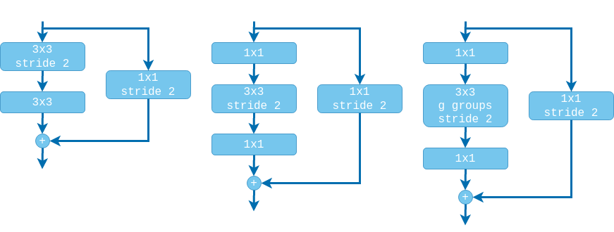
Note that if we are using the ‘pre-activation’ design then in the identity branch we need to add a batch norm and a relu layers before the $1 \times 1$ convolution.

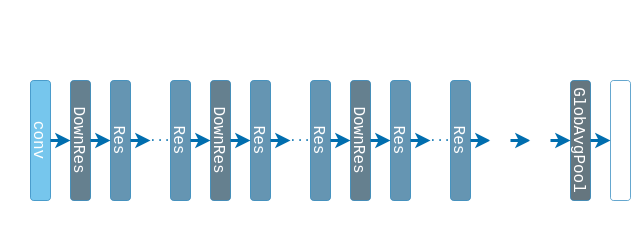
The final ResNet architecture consists of stacking ResBlocks, with occasionally downscaling the image with Downscale ResBlocks. After that a Global average pooling layer is applied as proposed in [⁷]. The original idea was to have the final convolution produce a tensor with the same number of channels as the number of classes, each channel corresponding to a confidence map for the given class. Replacing FC layers with global average pooling would not be as effective if were using linear convolutions instead of micro-networks. Later models, however, take a less extreme approach and add one more FC layer to scale the output to match the number of classes.

The number of stages should be such that the spatial dimensions of the tensor are reduced to approx. $8 \times 8$. For CIFAR-10, for example, we need 3 stages. For ImageNet what is done in practice is that the very first convolution is a $7 \times 7$ conv layer with stride of 2, scaling the input from $224 \times 224$ to $112 \times 112$. Then 4 stages are applied further reducing the size to $112 / 2^4 = 7 \times 7$.

However, we still need to choose the channels for each stage $C_1, C_2, C_3, \dots$, the blocks within each stage $B_1, B_2, B_3, \dots$, and also the groups within each block (if using ResNeXt blocks) $g_1, g_2, g_3, \dots$. Exploring the possible combinations to find the best solution is clearly infeasible, but there are a few guiding principles that we can use. The paper¹⁰ “Designing network design spaces” by Iliya Radosavovic et al. explores what the relation between these parameters should be, so that models at any scale would perform well. This lead to the design of the RegNet and the following principles:

1. Do not use any bottleneck.
2. Share the number of groups for all stages, i.e., $g_i = g \quad \forall i$.
3. Increase the number of channels across stages, i.e., $C_{i+1} \geq C_i$. In practice channels are usually doubled at every stage, however the authors report top performance at $C_{i+1} \approx 2.5 C_i$.
4. Increase the number of blocks in each stage, i.e., $B_{i+1} \geq B_i$, but not necessarily in the last stage. The pattern 1:1:3:1 is rather famous for networks with four stages.
5. Best performing models are usually around 20 blocks deep in total, and the other parameters are used to control the number of FLOPs.