An even more annotated Transformer

This post is based on the The annotated transformer and its older version. I decided to add some more annotations regarding the architecture of the transformer model¹ and why some specific design choices were made.

But first, a longer explanation about the attention layer in the transformer… If you don’t feel like reading then skip to the first code snippet or check out the full implementation on github.

ATTENTION⌗

What this layer does is it takes a sequence of elements $x_1, x_2, \dots, x_T$ and for every element $x_i$ produces an encoding $z_i$, that captures somehow the context of $x_i$, i.e., it is coupled with all other elements of the sequence. This operation is similar to the workings of an RNN, but the unrolling of an RNN is sequential and cannot be parallelized.

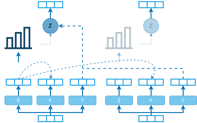
What we want to do is compute the encoding of $x_i$ independently, something like: $z_i = x_i W $, where $W$ is the encoding matrix. However, now $z_i$ is completely decoupled from the other sequence elements. The idea of the self-attention layer is to compute these independent encodings and then combine them. For every $x_i$ we compute a so called value encoding $v_i = x_i V$, and the final encoding $z_i$ is a weighted average of the value encodings of all the sequence elements:

$$ \displaystyle z_i = \sum_j \alpha_j v_j, $$

where $\alpha_j$ are the weights for the element $i$. But what should the values of those weights be? Well, we want to have a high value of $\alpha_j$ if element $i$ is closely realated to element $j$, i.e., element $i$ should “pay attention” to element $j$.

But we already have a proximity measure for vectors – we can simply take the scalar product: $\alpha_j = x_i x_j^{T}$. However, this implies that the attention score between $x_i$ and $x_j$ will be the same as the attention score between $x_j$ and $x_i$. Instead, we can take the attention score to be: $\alpha_j = x_i W x_j^{T}$, where $W$ is yet another encoding matrix. Now $x_i$ might pay a lot of attention to $x_j$, while the inverse does not need to be true. We go even a step further and define this encoding matrix as a product between two matrices, $W = Q K^{T}$. The attention score now becomes:

$$ \alpha_j = x_i Q K^{T} x_j^{T}. $$

We call the vector $q_i = x_i Q$ the query encoding of $x_i$, and the vector $k_j = x_j K$ the key encoding of $x_j$. All three matrices $Q, K, V$ are learnable parameters of the attention layer.

The weights for the weighted summation are obtained by simply applying a softmax on the attention scores. For the encodings $z_i$ we get:

$$ z_i = \text{softmax}(x_i Q K^T x^T) x V $$

The attention score $\alpha_j = q_i k_j^{T}$ will be high for keys that match the query $q_i$, and will be low for keys that do not match. What we are hoping to achieve is for our model to learn to map queries and their matching keys nearby in the embedding space.

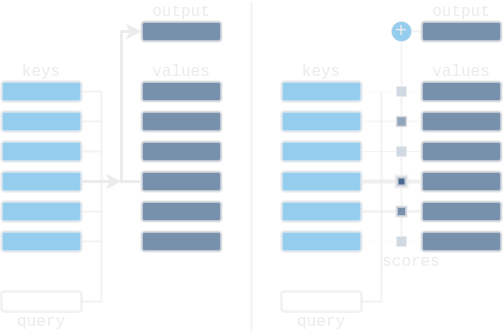
Continuing the query-key-value analogy, we can think of the attention layer as a soft lookup in a key-value store. In standard lookup tables the query matches one of the keys and the corresponding value is returned. In the soft lookup table the query matches all the keys softly, to a weight between 0 and 1. The values are then multiplied by the corresponding weights and summed to produce the output. In the self-attention layer the key-value store is built from the elements of the sequence, and then every element is matched with all the rest. In the cross-attention layer (used in the decoder) the key-value store is built from the source sequence processed by the encoder. Then every element from the target sequence is decoded by querying this key-value store like a memory database.

MULTI-HEAD ATTENTION LAYER⌗

One problem with the proposed self-attention mechanism is that an output $z_i$ will most likely be dominated by a single $v_i$, because the softmax quickly saturates. In order to have our $z_i$ “pay attention” to multiple $v_i$s we will use several sets of $Q$, $K$, and $V$ matrices. Each set is called an attention head, and the outputs of all the heads are concatenated at the end.

class MultiHeadAttention(nn.Module):
    def __init__(self, in_dim, qk_dim, v_dim, out_dim, n_heads, attn_dropout=0.):
        super().__init__()
        self.n_heads = n_heads
        self.dropout_p = attn_dropout

        self.Q = nn.Linear(in_dim, qk_dim, bias=False)
        self.K = nn.Linear(in_dim, qk_dim, bias=False)
        self.V = nn.Linear(in_dim, v_dim, bias=False)
        self.Wo = nn.Linear(v_dim, out_dim)
        self.attn_dropout = nn.Dropout(attn_dropout)

        nn.init.normal_(self.Q.weight, std=np.sqrt(2 / (in_dim + qk_dim//n_heads)))
        nn.init.normal_(self.K.weight, std=np.sqrt(2 / (in_dim + qk_dim//n_heads)))
        nn.init.zeros_(self.Wo.bias)

The initializer of the layer accepts the dimensionalities of the query, key and value spaces, and the number of heads. Note that the query and key must be in the same space in order to perform the dot product between the two. That is why a single parameter is provided for both.

In order not to increase the complexity of the model (i.e., number of params) when adding additional heads, the dimensionality of each head will be equal to the original dimensionality divided by the number of heads. Now, instead of defining the $Q$, $K$, $V$ layers for each head separately, we will define them once and split the result into separate heads later.

After the outputs of the heads are concatenated we will forward them through a final linear layer ($W_O$) in order to project them in the required output dimension.

Usually, for the transformer model we will initialize this layer as:

attn_layer = MultiHeadAttention(d, d, d, d, h)

which means that the output space will be the same as the input space, and the queries, keys and values will be projected by each head into a $(d//h)$-dimensional space.

Finally, we will specifically initialize the weights of the $Q$ and $K$ layers to be from a unit normal distribution with an std of $\sqrt{\frac{2}{\text{fan_in}+\text{fan_out}}}$, so that forwarding through these layers keeps the variance unchanged. Note that for $\text{fan_out}$ we use the per-head dimension, although I don’t think that this is all that important.

class MultiHeadAttention(nn.Module):
    def __init__(self, in_dim, qk_dim, v_dim, out_dim, n_heads, attn_dropout):
        # ...

    def forward(self, queries, keys, values, mask=None):
        B, T, _ = queries.shape
        _, Ts, _ = keys.shape
        if mask is not None: # unsqueeze the mask to account for the head dim
            mask = mask.unsqueeze(dim=1)

        q = self.Q(queries).view(B, T, self.n_heads, -1).transpose(1, 2) # X @ Q
        k = self.K(keys).view(B, Ts, self.n_heads, -1).transpose(1, 2)   # X @ K
        v = self.V(values).view(B, Ts, self.n_heads, -1).transpose(1, 2) # X @ V

        attn = torch.matmul(q, k.transpose(2, 3)) # XQ @ (XK)^T

        dk = k.shape[-1]
        attn /=  np.sqrt(dk)
        if mask is not None:
            attn.masked_fill_(~mask, -1e9)
        attn = torch.softmax(attn, dim=-1)  # shape (B, nh, T, Ts)
        attn = self.attn_dropout(attn)

        z = torch.matmul(attn, v)           # shape (B, nh, T, hid)
        z = z.transpose(1, 2).reshape(B, T, -1)
        out = self.Wo(z)                    # shape (B, T, out_dims)

        return out, attn

The forward pass accepts three different inputs, namely queries, keys and values. The usual way to call the self-attention layer is:

z, _ = attn_layer(x, x, x)

This will perform the self-attention operation described earlier. However, in some cases, e.g. in the decoder cross-attention layer, we want to compute our key embeddings and value embeddings not from $x$, but from a different sequence.

The forward pass is fairly straight forward. We first compute our query, key and value embeddings and then split them into separate heads. Then we calculate the attention scores and apply softmax to get the attention weights (probabilities). Before applying the softmax layer, however, we scale the scores by dividing by the dimensionality of the key embedding space. To see why this is done let’s assume that the keys and queries have zero mean and unit std. Then for the variance of the attention score between any query and key we get:

$$ \alpha = q_i k_j^T = \sum_{n=1}^{d_k} q_{in} k_{jn} $$ $$ \text{Var}(\alpha) = d_k $$ $$ \text{std}(\alpha) = \sqrt{d_k} $$

Applying softmax on the attention scores with such high variance will result in all of the weight being placed on one random element, while all the other elements will have a weight of zero. Thus, in order to have the attention scores with unit std, we scale by $\sqrt{d_k}$.

But is it safe to assume that our keys and queries have unit variance? Well, yes! The embeddings are computed by forwarding the input $x$ through the key and query layers. We can assume that the input already has unit variance by using a normalizing layer (e.g. LayerNorm), and the weights of the layers were initialized so that variance is preserved.

It looks strange that we are applying dropout directly to the attention probabilities just before performing the weighted summation. This means that our attention vector will most probably not sum to 1. The paper never mentions or explains this but it is used in the official implementation, including BERT and GPT. However, note that during evaluation dropout is not applied so we are probably fine.

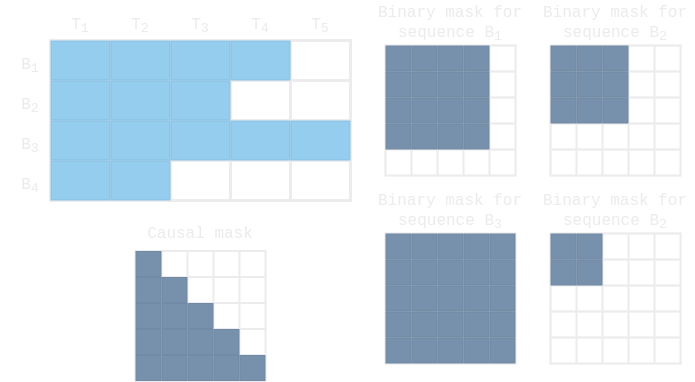
One final detail is the application of a mask over the attention scores. One reason why this is done is because the input to the attention layer is a batch of sequences, and not all sequences in the batch have the same length. Shorter sequences are padded, and the padded elements need to be masked so that they don’t take part in the attention score computation. In this case the mask is of shape $B \times T \times T$ and is different for every sequence of the batch. Another reason is for performing causal masking during decoding.

So why do we need both $Q$ and $K$ if we only ever use them in the form $Q K^{T}$ ? Except for making the query-key-value analogy more clear, is there any other reason to keep both matrices? We could just learn the product matrix $W = Q K^{T}$ ?

Well, yes, there is a reason.

If we were to learn only the product matrix then its size would be $D \times D$, while learning two separate matrices allows us to project into a lower-dimensional query-key space and now the size of each of the two matrices is $D \times d_k$, with $d_k « D$. Thus, we force the matrix $W = Q K^{T}$ to be not just any matrix, but a matrix with rank $d_k$.

Is this a reasonable thing to do?

Well, yes, it is.

Query and key embeddings don’t have to be in the large $D$-dimensional space. A smaller space could easily do the job, and it would prevent the model from overfitting.

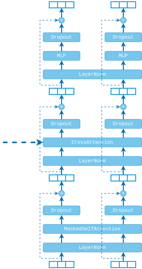
ENCODER BLOCK⌗

The encoder is a stack of $N$ identical blocks applied one after another. Each encoder block has a self-attention layer followed by a position-wise fully-connected network. Dropout is applied after each of the sub-layers followed by residual connection. The model also uses layer normalization.

class EncoderBlock(nn.Module):
    def __init__(self, d_model, n_heads, dim_mlp, dropout):
        super().__init__()

        self.attn = MultiHeadAttention(
            in_dim=d_model, qk_dim=d_model, v_dim=d_model, out_dim=d_model,
            n_heads=n_heads, attn_dropout=dropout,
        )
        self.attn_dropout = nn.Dropout(dropout)
        self.attn_norm = nn.LayerNorm(d_model)

        self.mlp = nn.Sequential(
            nn.Linear(d_model, dim_mlp), nn.ReLU(), nn.Linear(dim_mlp, d_model),
        )
        self.mlp_dropout = nn.Dropout(dropout)
        self.mlp_norm = nn.LayerNorm(d_model)

The initializer of the encoder block accepts the dimensionality of the model and the number of attention heads and defines all sub layers to produce outputs with the same dimension $d_{model}$ in order to facilitate the use of residual connections.

The residual connection is applied after both the self-attention and the fully-connected layers and its purpose is twofold:

1. Similar to ResNets, this residual connection allows us to continuously improve model performance by stacking more encoder blocks. If a deeper model wants to reproduce a shallower model, then we simply have to learn that the residual is $f(x)=0$.
2. However, more importantly, the residual connection preserves the positional information within the sequence. Without it this information would be lost after the first self-attention layer. Now each self-attention layer would have to learn this information based just on the input features, which is highly unlikely.

Another subtlety is the use of a fully-connected network. Since there are no elementwise non-linearities in the self-attention layer, stacking more self-attention layers would just re-average the value vectors. Thus, a small neural net is added after each self-attention layer to post-process each output vector separately. Usually this network is a two-layer MLP with inner dimensionality $2-8 \times d_{model}$. A wider shallow network allows for faster parallelizable execution than a deeper narrow network.

Why use an MLP, and not some other type of layer?

In the paper² “FastSpeech: fast, robust and controllable text to speech” by Ren et al., in their FFT block they use two convolutional layers instead. The motivation is that the adjacent embeddings are more closely related in the character/phoneme sequence in speech tasks, than in a word sequence.

class EncoderBlock(nn.Module):
    def __init__(self, d_model, n_heads, dim_mlp, dropout):
        # ...

    def forward(self, x, mask=None):
        if mask is not None: mask = mask.unsqueeze(dim=-1)
        x = self.attn_norm(x)
        z, _ = self.attn(x, x, x, mask=mask)
        z = x + self.attn_dropout(z)

        z = self.mlp_norm(z)
        r = self.mlp(z)
        r = z + self.mlp_dropout(r)

        return r

The forward pass accepts the input sequence of shape $B \times T \times d_{model}$ and an optional mask tensor of shape $B \times T$ that indicates which elements of the input should be take part in the computation.

Note that our attention layer expects the mask to be of shape $B \times T \times T$. Simply broadcasting would not produce the exact same mask that we described earlier. However, it achieves the same effect since we don’t really care what the padded elements are attending.

The block also incorporates a layer normalization layer, which also plays a very important role, making sure that inputs to the self-attention layer are normalized with zero mean and unit variance. There are two options for the position of the normalization layer. In the original paper it is placed after the residual connection, but more recent implementations re-arrange the layers and place it in the beginning of the block. Recent research³ suggests that when using this “Pre-LayerNorm” configuration we can train the model without the warm-up stage of the optimizer.

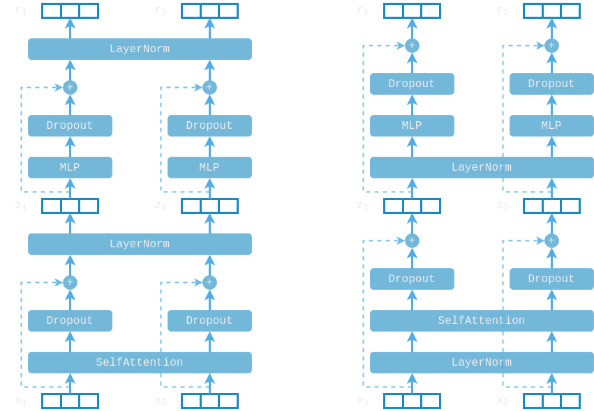
In this implementation we use the Pre-LN configuration, but note that now the final outputs of the encoder stack will not be normalized. To fix this we will add an additional LayerNorm layer after the final encoder block in the encoder stack.

DECODER BLOCK⌗

The decoder is a stack of $M$ identical blocks applied one after another.

class DecoderBlock(nn.Module):
    def __init__(self, d_model, n_heads, dim_mlp, dropout):
        super().__init__()
        self.self_attn = MultiHeadAttention(
            in_dim=d_model, qk_dim=d_model, v_dim=d_model, oug_dim=d_model,
            n_heads=n_heads, attn_dropout=dropout,
        )
        self.self_attn_dropout = nn.Dropout(dropout)
        self.self_attn_norm = nn.LayerNorm(d_model)

        self.cross_attn = MultiHeadAttention(
            in_dim=d_model, qk_dim=d_model, v_dim=d_model, out_dim=d_model,
            n_heads=n_heads, attn_dropout=dropout,
        )
        self.cross_attn_dropout = nn.Dropout(dropout)
        self.cross_attn_norm = nn.LayerNorm(d_model)

        self.mlp = nn.Sequential(
            nn.Linear(d_model, dim_mlp), nn.ReLU(), nn.Linear(dim_mlp, d_model),
        )
        self.mlp_dropout = nn.Dropout(dropout)
        self.mlp_norm = nn.LayerNorm(d_model)

The decoder block is actually very similar to the encoder block, but with two differences:

1. The self-attention layer of the decoder is actually masked self-attention, using a causal mask on the decoded sequence.
2. In addition to the two sub-layers, the decoder uses a third sub-layer, which performs cross-attention between the decoded sequence and the outputs of the encoder.

class DecoderBlock(nn.Module):
    def __init__(self, d_model, n_heads, dim_mlp, dropout):
        # ...

    def forward(self, x, mem, mem_mask=None):
        _, T, _ = x.shape
        causal_mask = torch.ones(1, T, T, dtype=torch.bool).tril().to(x.device)
        x = self.self_attn_norm(x)
        z, _ = self.self_attn(x, x, x, mask=causal_mask)
        z = x + self.self_attn_dropout(z)

        if mem_mask is not None: mem_mask = mem_mask.unsqueeze(dim=-2)
        z = self.cross_attn_norm(z)
        c, _ = self.cross_attn(z, mem, mem, mask=mem_mask)
        c = z + self.cross_attn_dropout(c)

        c = self.mlp_norm(c)
        r = self.mlp(c)
        r = c + self.mlp_dropout(r)

        return r

The forward pass accepts the target sequence of shape $B \times T_{tgt} \times d_{model}$ and the encoded source sequence of shape $B \times T_{src} \times d_{model}$.

The self attention layer operates on the target sequence using a lower-triangular boolean mask to prevent current elements from attending future elements. Since the target sequence is already masked with a causal mask we don’t need to provide any additional masking for it.

The cross attention uses the target sequence only for computing the query embeddings, and uses the encoded source sequences instead for computing the key and value embeddings. Now the key and value embeddings represent a memory database which the model queries during decoding.

Since the target sequence is attending the encoded source sequence, the cross-attention scores matrix for each sequence of the batch (and for each head) will be of shape $T_{tgt} \times T_{src}$. An optional mask can be provided for the encoded source sequence, which, again, needs to be broadcast to the correct shape, meaning that we’ll need to unsqueeze along the second dimension, instead of the last.

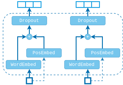
TOKEN EMBEDDING LAYER⌗

Note that both the encoder and the decoder layers accept input as sequences of vectors, meaning that we can use these layers for any problem where our data is already vector-encoded. However, if we want to apply these layers to language tasks we need to forward our tokens through an embedding layer, before feeding them to the transformer blocks.

One additional problem that we need to solve is that of encoding the order of the sequence, since the attention layers (and consequently the encoder block) are permutation-equivariant and have no notion of order.

class TokenEmbedding(nn.Module):
    def __init__(self, word_embed_weight, pos_embed_weight, scale, dropout):
        super().__init__()
        max_len, _ = pos_embed_weight.shape
        self.max_len = max_len
        self.word_embed_weight = word_embed_weight
        self.pos_embed_weight = pos_embed_weight
        self.dropout = nn.Dropout(dropout)

        self.register_buffer("positions", torch.arange(max_len).unsqueeze(dim=0))
        self.register_buffer("scale", torch.sqrt(torch.FloatTensor([scale])))

The initializer will directly accept the word embedding and the positional embedding matrices. This flexibility allows us to share the same positional embedding matrices for the source and target sequences. The original paper uses fixed positional embeddings by concatenating sine and cosine functions of different frequencies, so we can pass that as well if we want. However, we will be using randomly initialized positional embeddings that will be learned from scratch. We could also pass directly learned word embeddings if we want.

The paper also briefly mentions (see Sec. 3.4) that they will be using the same word embeddings for both the source and the target sequences. And, in addition, this same embedding matrix will be used for the final output layer of the decoder, citing previous research done here⁴.

Sharing the same embedding matrix for the source and target sequences makes, of course, total sense in some tasks like text summarization or question answering, where both sequences share the same vocabulary. But not so much in tasks like machine translation, where the vocabularies could be wildly different. Right? Well.. It turns out that if you are using a sub-word vocabulary and you are translating between english and french, or english and german, then around 85-90% of the sub-words are shared between the languages (see again [⁴]). So, yeah, maybe in these specific cases it makes sense, but otherwise – I don’t think so.

(I wonder why nobody reports translating between german and french :? Don’t sue me!)

Regarding sharing the same weight matrix between the target word embeddings and the decoder output layer. This reportedly improves model performance (see again [⁴]), but we have to be cautious with the initializations. Note that the outputs of the decoder are fed into a softmax layer, which could quickly saturate if these numbers have high variance. This means that the decoder output layer has to use some variance reduction initialization technique, like Xavier init. On the other hand, the embedding layer is essentially a table look-up, and so in order to keep variance constant, it should be initialized with zero mean and unit std. In addition, we will be summing the word embeddings with the positional embeddings, so they should be in the same scale.

What we will do is provide an additional scale parameter, which will be used to scale the word embeddings before adding them to the positional embeddings. Obviously, this scale parameter will depend on the initialization of the word embeddings and positional embeddings, whether we use sine and cosine positional encoding, whether we add or concatenate, and so on.. The original paper vaguely mentions that they are using a scale of $\sqrt{d_{model}}$, but honestly… no one knows why..

class TokenEmbedding(nn.Module):
    def __init__(self, word_embed_weight, pos_embed_weight, scale, dropout):
        # ...

    def forward(self, x):
        _, T = x.shape
        if T > self.max_len:
            raise RuntimeError("Sequence length exceeds the maximum allowed limit")

        pos = self.positions[:, :T]
        word_embed = F.embedding(x, self.word_embed_weight)
        pos_embed = F.embedding(pos, self.pos_embed_weight)
        embed = pos_embed + word_embed * self.scale
        return self.dropout(embed)

The forward pass simply looks up the word embeddings and the positional embeddings of the sequence elements. The word embeddings are then scaled and added to the positional embeddings. You could concatenate them as well, but people mostly just add them.

Note that the tensor with positions is registered as a module buffer, so it resides on the same device as the model parameters. When calling the forward function we don’t have to initialize a new tensor and push it to the gpu, but we can simply slice the buffer. However, slicing out of bounds on a cuda device might throw some very cryptic error messages, so we will explicitly verify that we don’t exceed the maximum sequence length.

TRANSFORMER⌗

Finally, let’s see how everything connects to construct the transformer model.

class Transformer(nn.Module):
    def __init__(
            self, src_vocab_size, tgt_vocab_size, max_seq_len,
            d_model, n_heads, n_enc, n_dec, dim_mlp, dropout,
        ):
        super().__init__()
        scale = np.sqrt(d_model)
        pos_embed = nn.Parameter(torch.randn(max_seq_len, d_model))
        src_word_embed = nn.Parameter(torch.randn(src_vocab_size, d_model) / scale)
        if tgt_vocab_size is None:
            tgt_word_embed = src_word_embed
        else:
            tgt_word_embed = nn.Parameter(torch.randn(tgt_vocab_size, d_model) / scale)

        self.src_embed = TokenEmbedding(src_word_embed, pos_embed, scale, dropout)
        self.tgt_embed = TokenEmbedding(tgt_word_embed, pos_embed, scale, dropout)
        self.tgt_proj_weight = tgt_word_embed

        self.encoder_stack = nn.ModuleList((
            EncoderBlock(d_model, n_heads, dim_mlp, dropout) for _ in range(n_enc)
        ))
        self.enc_norm = nn.LayerNorm(d_model)
        self.decoder_stack = nn.ModuleList((
            DecoderBlock(d_model, n_heads, dim_mlp, dropout) for _ in range(n_dec)
        ))
        self.dec_norm = nn.LayerNorm(d_model)

The initializer accepts the size of the source and target vocabularies, and initializes word embedding matrices for the source and target sequences. Note that the final decoder layer projecting back to the target vocabulary will use the same weights as the target word embeddings. No need to transpose the matrix because pytorch stores the weights of the linear layers in transposed form. The embedding weights are initialized from a normal distribution with zero mean and std equal to $1 / \sqrt{d_{model}}$ because of the sharing with the final output layer. The word embeddings will be scaled back with a factor of $\sqrt{d_{model}}$.

The positional embedding weights are initialized from a standard normal and are shared between the source and target embedding layers. Note that we need the maximum sequence length in order to initialize these embeddings. If the source and target sequences share the same vocabulary, then passing None for the size of the target vocabulary will share the same word embedding weights as well.

The encoder and decoder stacks use the same settings for initializing the blocks. Note that we also initialize two additional LayerNorm layers which are to be applied at the end of each stack because of the Pre-LN architecture.

class Transformer(nn.Module):
    def __init__(self, ...):
        # ...

    def encode(self, src, src_mask):
        z = self.src_embed(src)
        for encoder in self.encoder_stack:
            z = encoder(z, src_mask)
        return self.enc_norm(z)

    def decode(self, tgt, mem, mem_mask):
        z = self.tgt_embed(tgt)
        for decoder in self.decoder_stack:
            z = decoder(z, mem, mem_mask)
        return self.dec_norm(z)

    def forward(self, src, tgt, src_mask=None):
        mem = self.encode(src, src_mask)
        out = self.decode(tgt, mem, src_mask)
        tgt_scores = F.linear(out, self.tgt_proj_weight)
        return tgt_scores

The forward pass accepts a source sequence of shape $B \times T_{src}$ and a target sequence of shape $B \times T_{tgt}$. An optional mask for the source sequence can be provided with the same shape, indicating which elements should take part in the calculation. The output will be a tensor of shape $B \times T_{dec} \times D_{vocab}$ assigning to each position of the target sequence a vector of scores over the target vocabulary. Note that the forward pass uses teacher forcing and feeds the decoder the next true token instead of the one the model suggests.

We first encode the source sequence by running it through the encoder stack. An additional LayerNorm layer is applied because of the Pre-LN architecture. The target sequence is then forwarded through the decoder stack. The final encodings of the source sequence are fed as key-value memory to each of the decoder blocks. Again we normalize the decoder output and apply the final projection layer to produce scores over the target vocabulary.

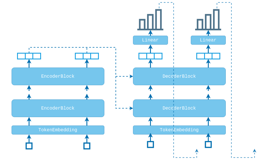
Note that we are feeding the final source sequence encodings to each of the decoder blocks, which means that each decoder can only query the final, most abstract embeddings of the source sequence. Another approach would be to connect each encoder block with its corresponding decoder block, much like a U-net. This way the decoder blocks lower in the stack would query earlier embeddings, which might be carrying useful information. That would require having the same number of encoder and decoder blocks in the two stacks, but I think this is the most common choice anyway.

Of course, you could just go all in and stack the outputs from all of the encoder blocks together and feed them to each and every decoder block. You would have to forward them through an additional linear layer to reduce the dimensionality back to $d_{model}$, or adjust the attention layer to accept key-value memory with dimension different from the query dimension. Anyway, I have never seen anyone do that and also I just made that up, so maybe don’t do it.

INFERENCE⌗

In order to generate a sequence during inference we will use a simple greedy decoding strategy. (Maybe I will add beam search at some point.)

class Transformer(nn.Module):
    def __init__(self, ...):
        # ...

    def encode(self, src, src_mask):
        # ...

    def decode(self, tgt, mem, mem_mask):
        # ...

    def forward(self, src, tgt, src_mask=None):
        # ...

    @torch.no_grad()
    def greedy_decode(self, src, src_mask, bos_idx, eos_idx, max_len=80):
        B = src.shape[0]
        done = {i : False for i in range(B)}
        was_training = self.training
        self.eval()

        tgt = torch.LongTensor([[bos_idx]] * B).to(src.device)
        mem = self.encode(src, src_mask)
        for _ in range(max_len-1):
            out = self.decode(tgt, mem, mem_mask=src_mask)
            scores = F.linear(out, self.tgt_proj_weight)
            next_idx = torch.max(scores[:, -1:], dim=-1).indices
            tgt = torch.concat((tgt, next_idx), dim=1)

            for i, idx in enumerate(next_idx):
                if idx[0] == eos_idx: done[i] = True
            if False not in done.values(): break

        if was_training: self.train()
        return tgt

The decoding function takes as argument the source sequence to be decoded and the start and end tokens. We will first encode the source sequence by running it through the encoder stack and then we will prompt the decoder with the start token to start generating. The decoded sequence will be generated one element at a time. At every step of the loop we feed the decoder the entire target sequence that has been generated until now. For each element the decoder will output scores over the target vocabulary indicating which should be the next element. We are only concerned with the scores for the last element of the sequence, because they are used to predict the next element. Decoding continues until the end token is produced.

Since we are decoding a batch of sequences, we need to continue iterating until every sequence in the batch has been decoded. To keep track of that we will simply update a dict indicating which sequences are done.

Note that the provided tokens for beginning of sequence (bos) and end of sequence (eos) don’t have to be the special <START> and <END> tokens. We could try to start the sequence with any item from the vocabulary. We could also try to end the sequence with any item, but keep in mind that the model was trained to end sequences specifically with the <END> token.

SO? DOES IT WORK?⌗

To quickly test the code we will try to learn a simple task: reversing the order of a sequence.

from torch.nn.utils.rnn import pad_sequence

device = torch.device("cuda" if torch.cuda.is_available() else "cpu")
bos_idx, eos_idx, pad_idx = 1, 2, 0
vocab_size, src_len = 100, 16

data_loader = data.DataLoader(  # random sequences of different lengths
    dataset=[torch.randint(3, vocab_size, (randint(src_len//2, src_len),)) for _ in range(50000)],
    batch_size=128, shuffle=True, drop_last=True,
    collate_fn=lambda batch: (
        pad_sequence(batch, batch_first=True, padding_value=pad_idx),
        pad_sequence(           # flip the sequence and add <START> and <END> tags
            [torch.LongTensor([bos_idx] + x.flip(0).tolist() + [eos_idx]) for x in batch],
            batch_first=True, padding_value=pad_idx,
    )),
)

The dataset will consist of 50000 random sequences of numbers with varying lengths between 8 and 16 elements. The target sequence is simply the reversed sequence nested between <START> and <END> tags. The data loader will generate random batches from the training set and will automatically pad shorter sequences to match the length of the longest sequence in the batch.

transformer = Transformer(
    src_vocab_size=vocab_size, tgt_vocab_size=None, max_seq_len=32,
    d_model=64, n_heads=2, n_enc=2, n_dec=2, dim_mlp=128, dropout=0.1,
).to(device)
optim = torch.optim.AdamW(transformer.parameters(), lr=1e-3, weight_decay=1e-4)

for _ in range(10):
    for src, tgt in data_loader:
        src, tgt = src.to(device), tgt.to(device)
        tgt_in, tgt_out = tgt[:, :-1], tgt[:, 1:]
        logits = transformer(src, tgt_in, (src != pad_idx))
        loss = F.cross_entropy(logits.permute(0,2,1), tgt_out, ignore_index=pad_idx)

        optim.zero_grad()
        loss.backward()
        torch.nn.utils.clip_grad_norm_(transformer.parameters(), 1.)
        optim.step()

x = torch.LongTensor([3, 5, 8, 13, 21, 34, 55, 89]).unsqueeze(dim=0).to(device)
y = transformer.greedy_decode(x, None, bos_idx, eos_idx, max_len=32)
print(y)
>>> [1, 89, 55, 34, 21, 13, 8, 5, 3, 2]

We will use a relatively small model for this simple task. Since both the source and the target sequences come from the same vocabulary, we will share the word embedding matrices by setting tgt_vocab_size=None. Note that during training we feed all but the last element of the target sequence. We don’t want to feed the <END> token, we only want the model to predict it. When computing the loss we compare the predictions of the model with all but the first element of the target sequence. To generate the mask for the source sequence we will simply compare each source token with the <PAD> tag.

MACHINE TRANSLATION⌗

Finally, let us consider a more realistic example using the Multi30k German-English translation dataset.

from torch.nn.utils.rnn import pad_sequence
from torchtext.datasets import Multi30k
from torchtext.data.utils import get_tokenizer
from torchtext.vocab import vocab

train_data = Multi30k(root="datasets", split="train")
train_data = [(src, tgt) for src, tgt in train_data if len(src) > 0]

UNK, PAD, BOS, EOS = ("<UNK>", "<PAD>", "<START>", "<END>")
tokenizer = get_tokenizer("basic_english")
en_counter, de_counter = Counter(), Counter()
for src, tgt in train_data:
    en_counter.update(tokenizer(src))
    de_counter.update(tokenizer(tgt))
de_vocab = vocab(en_counter, specials=[UNK, PAD, BOS, EOS])
de_vocab.set_default_index(de_vocab[UNK])
en_vocab = vocab(de_counter, specials=[UNK, PAD, BOS, EOS])
en_vocab.set_default_index(en_vocab[UNK])
pad_idx = de_vocab[PAD] # pad_idx is 1
assert en_vocab[PAD] == de_vocab[PAD]

We will use a very basic english tokenizer for both languages. We will also use the torchtext vocab object to create a vocabulary that supports mapping from tokens to indices and vice-versa.

lengths = [len(src) for src, _ in train_data]
batch_size = 128
train_loader = data.DataLoader(
    dataset=train_data,
    batch_size=batch_size, shuffle=True, drop_last=True,
    collate_fn=lambda batch: (
        pad_sequence(
            [torch.LongTensor(de_vocab(tokenizer(x))) for x, _ in batch],
            batch_first=True, padding_value=pad_idx),
        pad_sequence(
            [torch.LongTensor(en_vocab([BOS] + tokenizer(y) + [EOS])) for _, y in batch],
            batch_first=True, padding_value=pad_idx),
    ),
    num_workers=4,
)

When initializing the data loader we will provide a collate function that will tokenize and then pad the src and tgt sequences. For the tgt sequence we also add the <START> and <END> tokens.

transformer = Transformer(
    src_vocab_size=len(de_vocab), tgt_vocab_size=len(en_vocab), max_seq_len=256,
    d_model=256, n_heads=8, n_enc=4, n_dec=4, dim_mlp=512, dropout=0.1,
)
transformer.to(device)
optim = torch.optim.AdamW(transformer.parameters(), lr=1e-4, weight_decay=1e-4)

for e in range(30):
    for src, tgt in train_loader:
        src, tgt = src.to(device), tgt.to(device)

        # Forward pass.
        tgt_in, tgt_out = tgt[:, :-1], tgt[:, 1:]
        src_mask = (src != pad_idx)
        logits = transformer(src, tgt_in, src_mask)
        loss = F.cross_entropy(logits.permute(0,2,1), tgt_out, ignore_index=pad_idx)

        # Back-prop.
        optim.zero_grad()
        loss.backward()
        torch.nn.utils.clip_grad_norm_(transformer.parameters(), 1.)
        optim.step()

sent = ["zwei", "frauen", "spazieren", "und", "lachen", "im", "park", "."]
x = torch.LongTensor(de_vocab(sent)).unsqueeze(dim=0).to(device)
y = transformer.greedy_decode(x, None, en_vocab[BOS], en_vocab[EOS])
print(en_vocab.lookup_tokens(y[0].tolist()))
>>> ['<START>', 'two', 'women', 'are', 'walking', 'and', 'laughing', 'in', 'the',
     'park', '.', '<END>']

The dataset is fairly small so we won’t need a big model. Using these settings the model has $12.5M$ params, and in only 30 epochs (20 mins on may laptop) it learns to generate some decent looking translations.

TRICKS: BATCHING BY LENGTH⌗

When sampling batches we actually want to have sequences with similar lengths in each batch, so that there is minimum padding. For this reason we will provide our own batch sampler that does that.

class BatchSampler:
    def __init__(self, lengths, batch_size):
        self.lengths = lengths
        self.batch_size = batch_size

    def __iter__(self):
        size = len(self.lengths)
        indices = list(range(size))
        random.shuffle(indices)

        step = 100 * self.batch_size
        for i in range(0, size, step):
            pool = indices[i:i+step]
            pool = sorted(pool, key=lambda x: self.lengths[x])
            for j in range(0, len(pool), self.batch_size):
                if j + self.batch_size > len(pool): # assume drop_last=True
                    break
                # Ideally, there should also be some shuffling here.
                yield pool[j:j+self.batch_size]

    def __len__(self):
        return len(self.lengths) // self.batch_size

The batch sampler is initialized by providing a list with the lengths of each of the sequences in the dataset. During iteration, the sampler will hold a pool of sequence indices sorted by sequence length. Each batch will be drawn from the sorted pool, thus reducing the amount of padding. We chose here the pool to be $100 \times$ the batch size, but for other tasks a different setting might work better. Note that we are also implementing the __len__ method, which would allow us to call len() on the data loader.

train_loader = data.DataLoader(
    dataset=train_data,
    # batch_size=batch_size, shuffle=True, drop_last=True,
    batch_sampler=BatchSampler(lengths, batch_size),
    collate_fn=lambda batch: (
        pad_sequence(
            [torch.LongTensor(de_vocab(tokenizer(x))) for x, _ in batch],
            batch_first=True, padding_value=pad_idx),
        pad_sequence(
            [torch.LongTensor(en_vocab([BOS] + tokenizer(y) + [EOS])) for _, y in batch],
            batch_first=True, padding_value=pad_idx),
    ),
    num_workers=4,
)

sum((x == pad_idx).sum() / x.shape[0] for x, _ in train_loader) / len(train_loader)
>>> 15.25 # when no special batching
>>> 3.62  # with our batch sampler

When initializing the data loader, instead of providing the batch size parameter, we will pass an instance of our batch sampler. To measure the effectiveness of our batch sampler we will calculate the average number of pads per sequence.